CE 541: Introduction to SEEPW for geotechnical seepage modeling

Last Updated: 2020-10-29

Geotechnical Seepage Modeling

2D seepage modeling is valuable in many engineering applications. Geotechnical engineers use seepage modeling to estimate groundwater flows through structures, or to evaluate stability of water retention structures. Environmental engineers use seepage modeling to analyze contaminant transport or infiltration through landfill covers, for example.

There are three main objectives from geotechnical seepage models:

- seepage rates (e.g., how much flow is expected into an excavation?)

- pore water pressures (important for , of course)

- exit gradients (high exit gradients == erosion and instability)

What will you learn in this exercise?

In this exercise, you will be introduced to 2D seepage modeling in SEEPW. Throughout the lesson, a dam seepage model will be constructed and then you will examine how seepage flow through the dam changes as hydraulic conditions change.

This lesson includes:

Defining model geometry,
Defining and assigning soil material models,
Defining and assigning boundary conditions,
Checking model convergence, and
Analyzing simulated results.

The example problem will be addressed throughout this document. The example problem material will be presented in green boxes.

Tips for numerical analysis

Following some general guidelines when performing numerical analysis will help you achieve high-quality results, as well as document and evaluate your results.

Organize a harddrive or a cloud directory for your numerical analysis project. Include different folders for (i) saving model scenario results, (ii) compiling and reporting your results, (iii) keeping old versions of the model that work but you have since updated, (iv) documenting changes and updates you make.
Garbage in = garbage out. This is true for any type of analysis. The model parameters (e.g., geometry, soil properties, material parameters) must be reasonable for the result to be reasonable.
Critically evaluate your model results. Think about whether your results make sense and are what you expected. Can you explain your results based on geotechnical engineering principles? A great way to do this is to do a first-order analysis (e.g., draw a flownet) and see how closely your results agree.
Understand the model. Models should not be a blackbox, meaning that you should understand how your inputs are processed to deliver the model outputs. This can take time, but it is absolutely worthwhile if you will often be working with a certain model.

Step 1: Download & Install Geo-Studio (skip to the next step if you are using a CE lab computer)

GeoStudio download

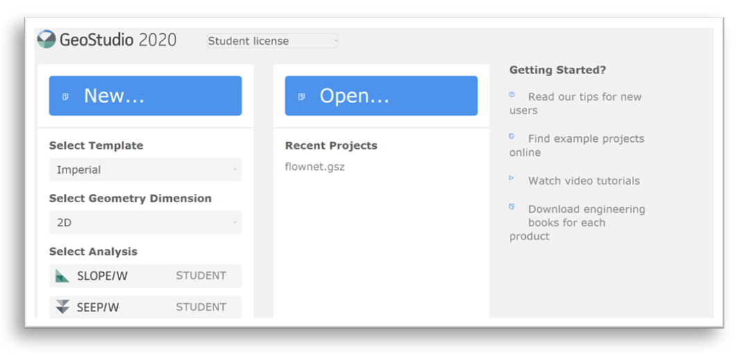
Step 2: Start SEEP/W with a Student License

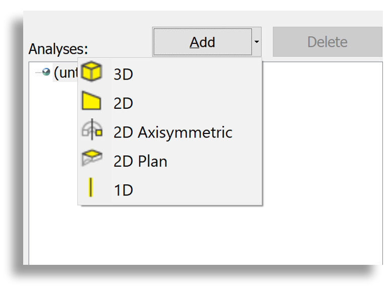
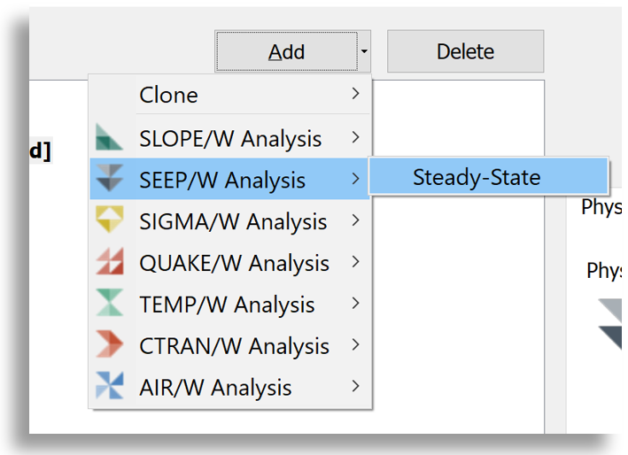
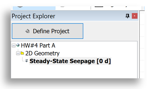
Step 3: Add a New Analysis

In the Define Project pane, add a new analysis by selecting the appropriate geometry. You may also need to define an analysis.
Once the new analysis is created, save the file in your project folder with an appropriate name.

Step 4: Select Units and Grid View

Units

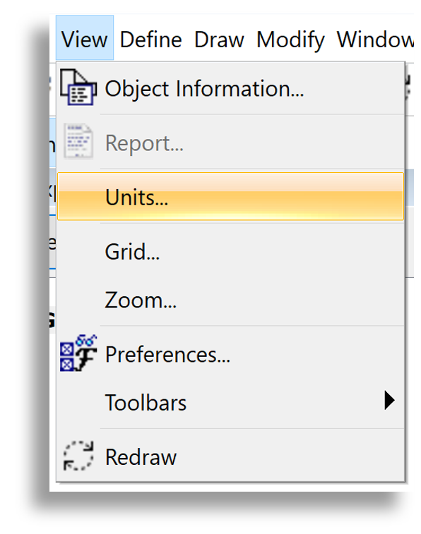
Units can be changed by selecting view-->units

Grid

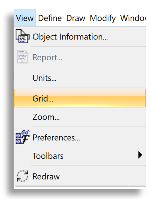
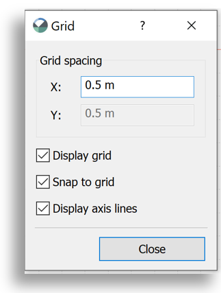
The view grid spacing and options can be changed with view-->grid. It can be useful when drawing the geometry to adjust the background grid based on the problem's geometry.

Remote Connection for Geostudio

GeoStudio is available in the EB-325 and FAB 55-17 MCECS computer labs.

https://intranet.cecs.pdx.edu/remote_lab/

Model geometry is made up of points, lines and regions. You can either:

Draw geometry where you draw the geometry directly on the grid
Define geometry where you put the coordinates of points in directly, and define lines and regions based on points.

Draw Points

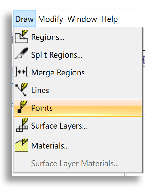
Points outline the corners or breaks in your model's geometry. To place points, select Draw->Points, then click on the grid where points should be.

Draw Lines

Lines connect two model points. The lines will define model and material boundaries. Boundary conditions will be assigned along the lines.

Draw the lines by selecting draw-->lines and clicking to connect two points.

You can edit the points that define a line with the define-->lines option.

Draw Regions

Regions will be defined by specifying lines that define a region. Material models will be assigned to each region.

Draw the regions with draw-->region and outline regions that will have a single material model.

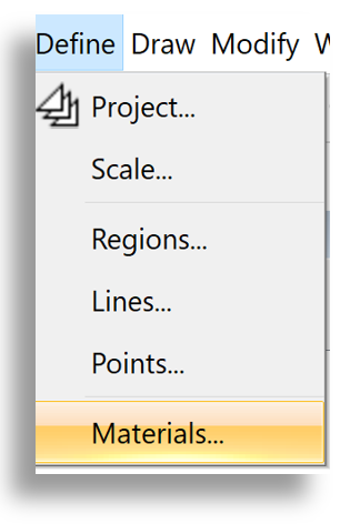
Defining Material Models

We need to use different material models to capture hydraulic conductivity and to assign hydraulic properties. Defining material models will allow us to associate different hydraulic conductivities with different soil types.

Select Add in the Define Materials window. Suggest that the name is either the soil type or name of the soil unit. For example, "silty clay" or "Columbia River alluvium" will provide more information than "unit 1".
Specify a name and color for a soil in your model.
Select a saturated or saturated/unsaturated soil model.
Fill in the model properties for your material model.

Selecting material properties

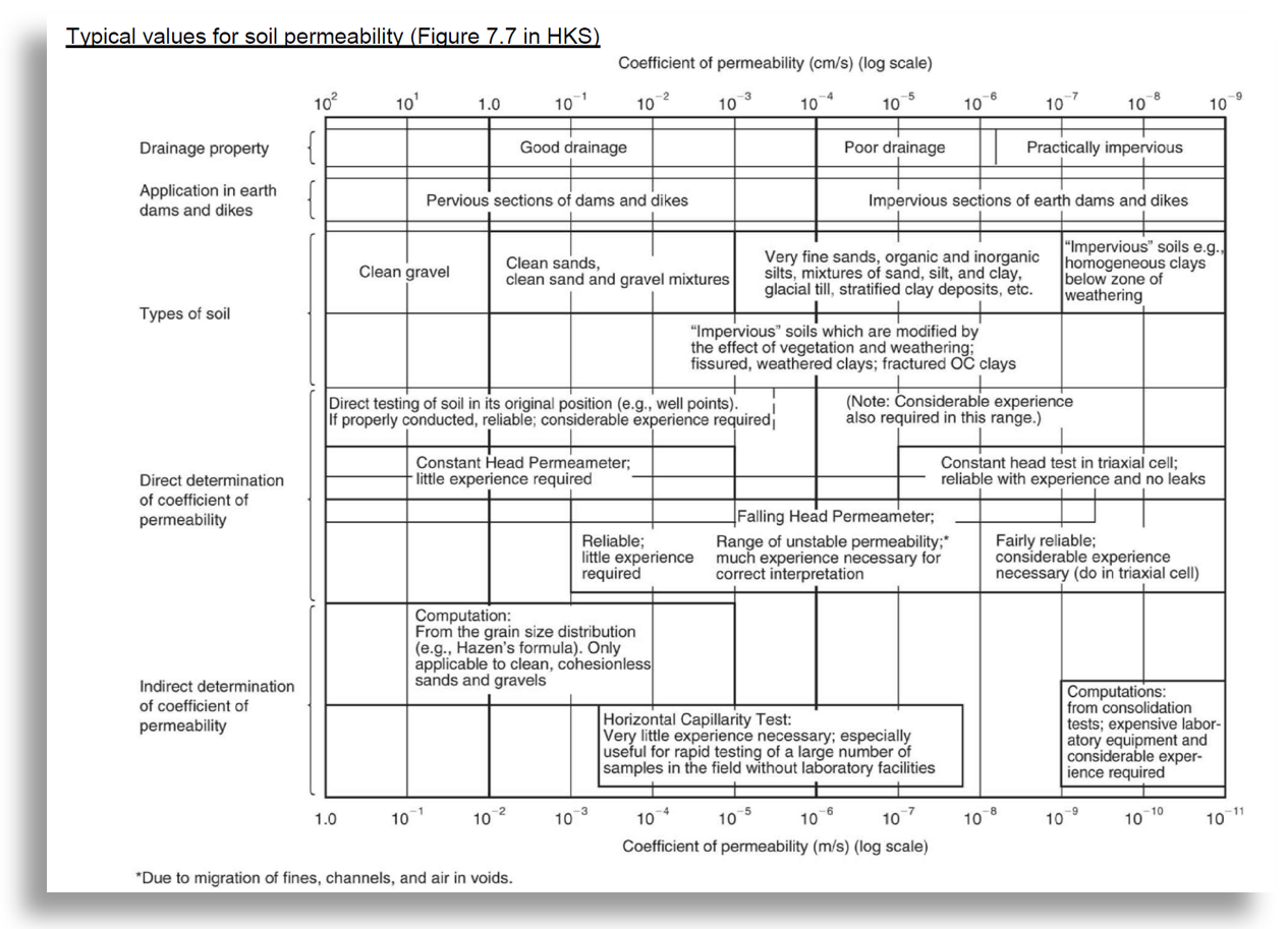
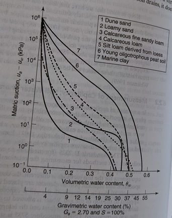
Figure 6.8 in Holtz Kovac & Sheahan (2011)

Table 3.4 from Powrie (2015)

Soil name	θs	θr
Hygiene sandstone	0.250	0.153
Touchet silt loam	0.469	0.190
Guelph loam (drying)	0.520	0.218
Guelph loam (wetting)	0.434	0.218
Bei netofa clay	0.446	0

Levee example - material models: For this example, we will need to use the saturated/unsaturated model. This means that the model will account for how hydraulic conductivity decreases as Sr decreases.

You will need three material models for the clayey sand, silty sand, and silty gravel soils. This example is only going to go through the clayey sand unit.

Name the soil unit Clayey sand and select a saturated/unsaturated material model

Select "..." beside the Vol. Water Content Fn: selection. There will be a new Define Vol. Water Content Functions window that appears
Select Add in the Define Vol. Water Content Functions window. This will let you add a function that relates θ to u. Name the new function "Clayey sand".
In the Types selection list, select Vol WC Data Point Function. The other types are reasonable, but we will use this one for this example.
Select the Estimate button. A new window will appear.
In the new window, enter the saturated volumetric water content for clayey sand, and select a sample material.

Press OK and a volumetric water content function will be plotted. You can adjust the x and y-axes to get a better look at the function. When you understand the plots, select close.

In the Define Materials window, under the Vol. Water Content Fn: list, select the Clayey sand function that you just defined.
Now select the "..." next to the Hyd. Conductivity Fn list. A new Define Hydraulic Conductivity Functions window will appear.
Name the new function "Clayey sand" and select the Estimate button. A new window will appear.
Choose "Van Genuchten" as the Estimation Method.
Select the "Clayey sand" function for Vol. Water Content Fn.
Enter a saturated horizontal hydraulic conductivity value for Saturated Kx
Enter a Residual Water Content value. When everything is entered select OK.

The relationship between Kx and u is now plotted. Note that the x-axis plots - u values (u < 0 is suction). After you understand the plots, select Close.
You can change the Anisotropy of hydraulic conductivity in the Ky'/Kx' Ratio space. For isotropic hydraulic conductivity Ky/Kx = 1.
Now select the Clayey sand relationship you just defined in the Hyd. Conductivity Fn list.

Now the material model for Clayey sand has been defined. You can add additional materials with the Add button in the Define Materials window. You will also need to develop material models for the silty sand and silty gravel.

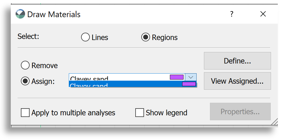
Assigning Materials to the Model

In this step you select what materials will be represented in each region of the model.

Select Draw-->Materials. In the Draw Materials window, select the material model you want to assign then click the region you want to assign that material to.

Defining Boundary Conditions

Select Define-->Boundary Conditions and the Define Boundary Conditions will appear.

Select Add-->New Hydraulic BC in the Define Boundary Conditions window.
Name the new BC and select the colour.
Select the Kind of boundary condition.

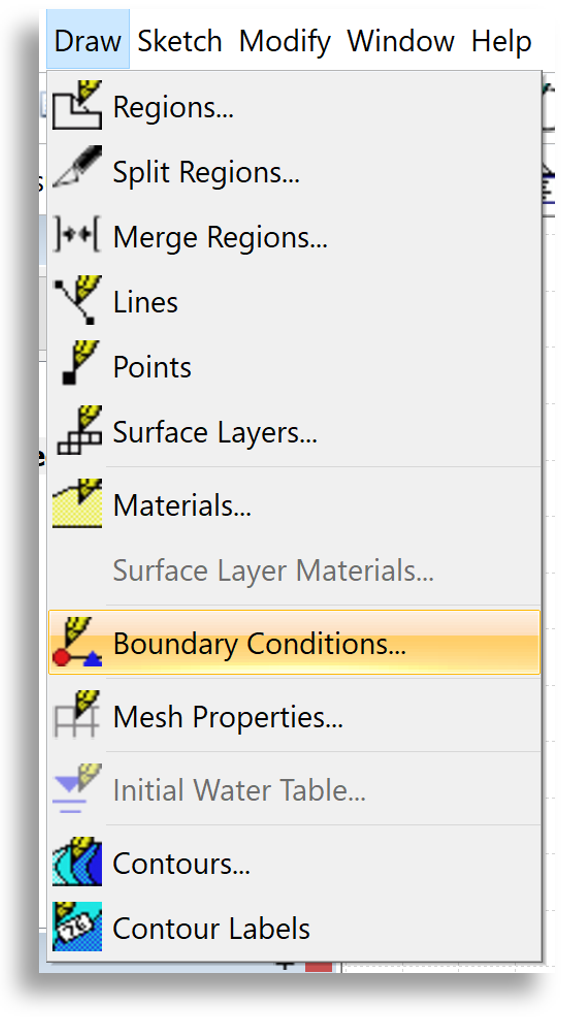
Assigning Boundary Conditions

Select Draw-->Boundary Conditions. With the appropriate BC selected from the Assign menu, apply the BC to the desired Line, Region, or Point.

We are going to solve the steady-state model. The solution works through iterations to converge on a steady-state solution of Heads and Fluxes at model nodes.

The Head and Flux at a model node is governed by Bernoulli's equation and Darcy's Law.

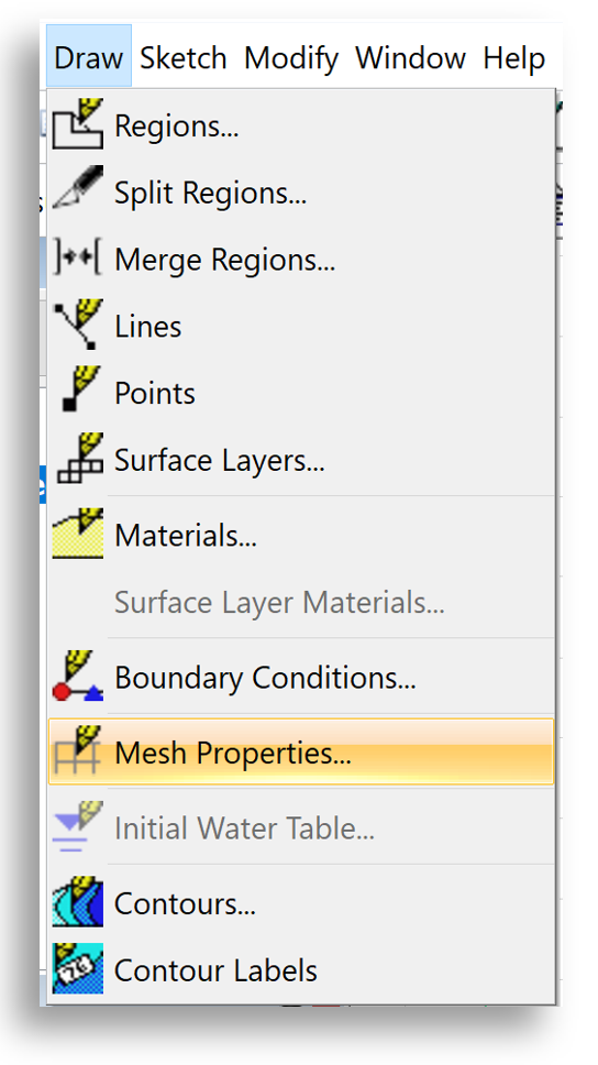
Generate the Mesh

The model builds elements defined by 4 nodes. In the model you have control of the mesh discretization to a certain extent: the Student License limits the model to 500 elements. SeepW will automatically build the mesh based on the specified element size.

To change the mesh discretization select Draw-->Mesh Properties. Input the Approximate Global Element Size, press enter and the mesh will automatically regenerate.

Select Solve Parameters

The numerical solve parameters can be checked and changed before solving the problem. To select the parameter select the Define Project button.

Select the Water tab. This tab allows you to specify many different solve parameters and to change some of the water parameters.

The model iterates through Head values at model nodes to find a solution. Convergence is determined when:

the pressure head difference between subsequent iterations is smaller than the Max. Pressure Head Difference, and
subsequent iterations are the same to the Significant Digits Equal value.

Start Solver

In the Solve Manager pane, select the Start button.

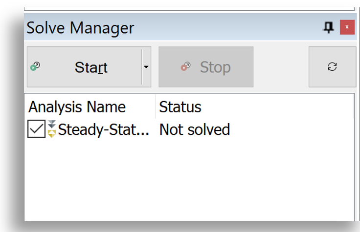
If the solution is successful, it will automatically go to the Results tab.

Checking Convergence

Check the convergence by selecting View-->Preferences. In the Preferences select Node Convergence.

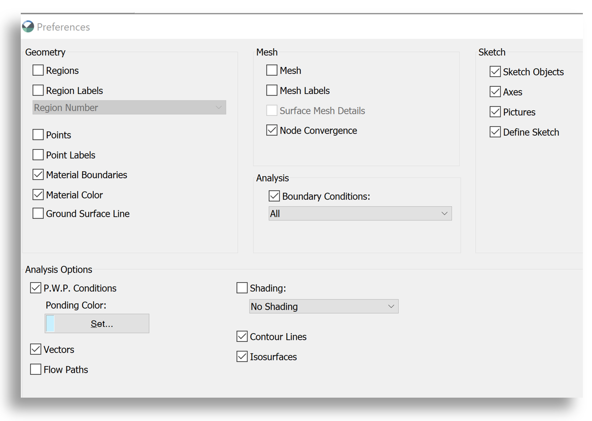
You can also plot the number of unconverged nodes versus iterations.

In the Results pane, select Draw Graph.
Add a new graph and give it a name.
In the Kind list, select Convergence (each iteration).
This will plot the unconverged pressure head nodes versus the iterations.

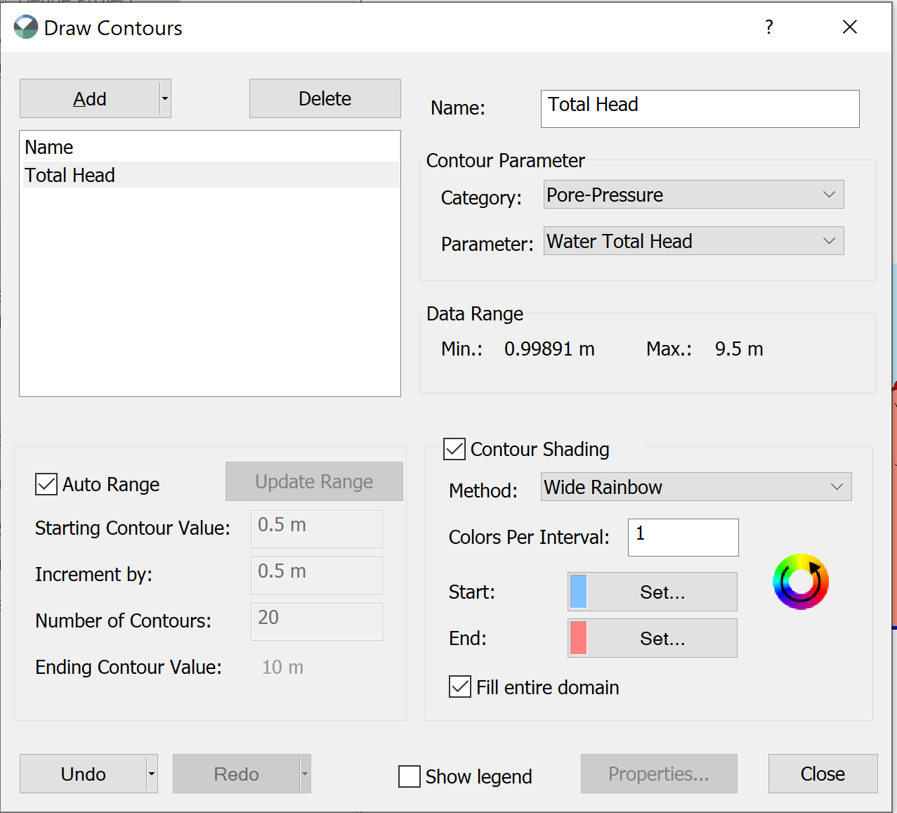
Contours

You can plot contours in the Solution pane by selecting the Contour button or selecting Draw-->Contours. The Draw Contours window should appear.

Select Add to add a new contour plot.

You can also add labels to the contour by selecting the label button.

Flow lines can be added by selecting the Flow Lines button and then clicking at points on the plot.

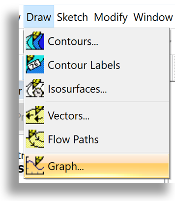
Graphs

Make plots within the solution by selecting Draw--> Graph in the Solution Pane.

Spatial plots can be made along lines, points, or regions in the model. You can make these by selecting Mesh in the Kind list, and then pushing the Set Locations button.