Last Updated: 2020-01-11
References: FLAC 8.1 Manual: User's Guide Problem Solving with FLAC; Command Reference; Fish in FLAC
This tutorial will provide background on the types of boundary conditions available in FLAC, and how these boundary conditions are implemented and changed when using FLAC.
What are model boundaries?
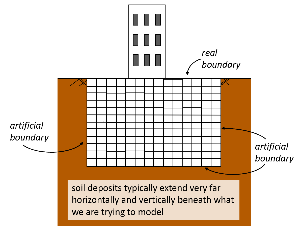
Boundary conditions are applied at the boundaries of models. So, in order to determine what boundary conditions best represent your problem, we first have to define what model boundaries are. Model boundaries can be either real or artificial.
- Real boundaries are those that physically exist for the modeled problem.
- Artificial boundaries are those that we approximate to simplify the problem. For geotechnical models, the bottom boundary is often an artificial boundary since soil and rock extend very deep below the ground surface. For example, instead of modeling the full extent of soil beneath a building, a modeller will choose a depth far enough beneath the building to act as the bottom boundary of the model.
Types of boundary conditions
There are two main types of boundary conditions that we will discuss: displacement-controlled and stress-controlled.
- Displacement-controlled prescribes gridpoint displacement at the boundary. This includes not allowing the boundary to move, or programming the boundary to displace a specific direction and distance during the simulation.
- Stress-controlled applies a stress across boundary gridpoints.
What you'll learn
- How to apply displacement controlled boundary conditions
- How to apply stress or force controlled boundary conditions
- How to determine appropriate boundary conditions
- Boundary conditions for simulating 1D compression, isotropic compression, and triaxial loading conditions
This tutorial does not discuss groundwater flow boundary conditions. These will come in future classes!
Displacement-controlled boundaries are applied at the model gridpoints. Essentially, you are telling the gridpoint how to move. But, instead of directly applying a displacement, you are applying a velocity at the gridpoints.
The displacement-controlled boundary condition is specified with the fix command.
For example:
fix x y j=1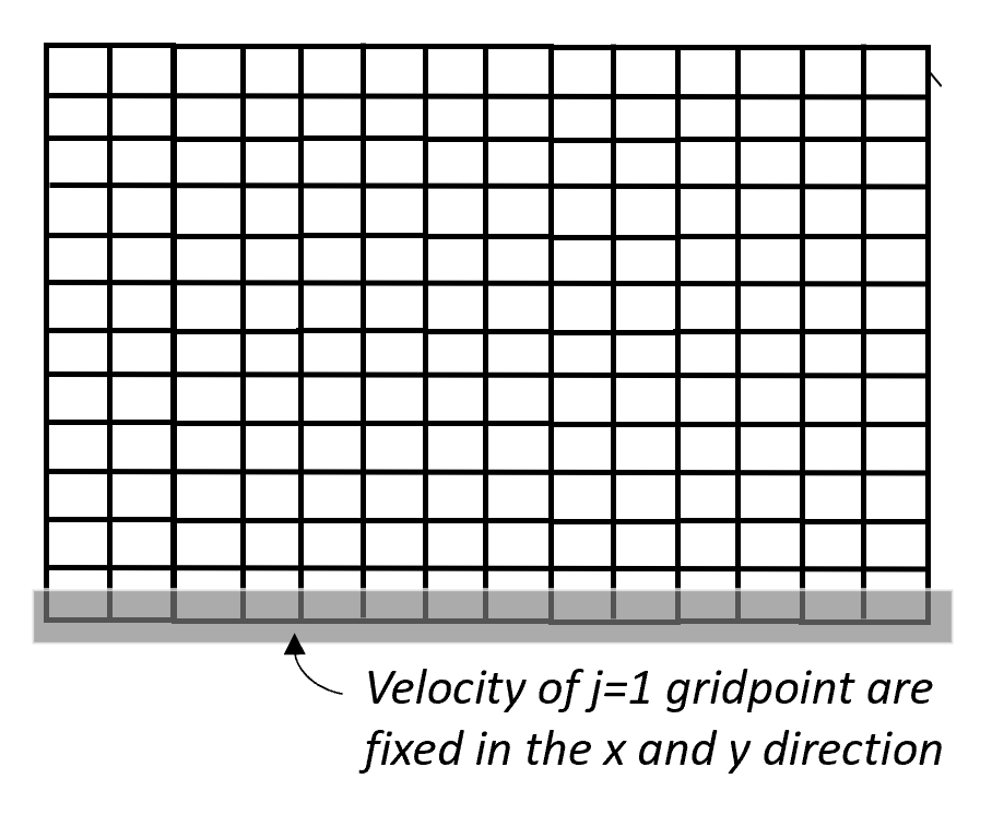
This tells FLAC the type of boundary condition (displacement-controlled), the direction of the boundary conditions (in both the x and y-directions), and the location of the boundary (at all gridpoints where j=1).
Applying boundary velocity
Once the fix command is given to FLAC, the velocity applied at those gridpoints should be specified.
The velocity sign conventions are:
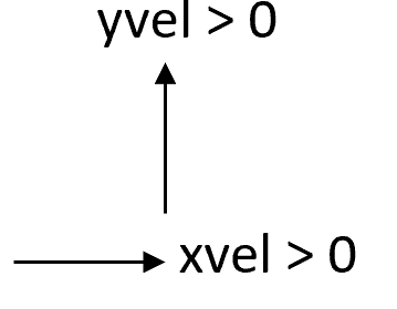
Velocities can be assigned with the initialize (ini) command or by assigning velocities through a FISH user-defined function.
Initialize command
The initialize command will assign velocities to gridpoints through a FLAC command. This is useful if velocities are not changing throughout the simulation.
fix x y j=1
ini yvel 0.1 j=1
ini xvel 0. j=1
This series of commands will apply a y-velocity of 0.1 along bottom gridpoints, and keeps the gridpoints fixed in the x-direction.
Assign velocities in FISH function
The fish functions can be useful if you want to change the velocity throughout the simulation. This is most useful if you need to ramp-up or ramp-down velocities.
For example, a fish function to increase the applied y-velocity along bottom gridpoints and keep the gridpoints fixed in the x-direction:
fix x y j=1   ;;; displacement boundary condition at bottom gps

def $ramp_up_velocity
   $y_vel_max = 0.1
   $intervals = 100

   loop $k (1,$intervals)
       $y_vel = $y_vel_max*($k/$intervals)

       $j = 1
       loop $i (1,gpi)
           yvel($i,$j) = $y_vel
          xvel($i,$j) = 0.
       end_loop
    end_loop
end
$ramp_up_velocity No-displacement boundaries
No-displacement boundaries are a type of displacement-controlled boundary. For no-displacement boundaries, the gridpoints are fixed in place.
For example:
fix x y i=1
ini yvel 0. i=1
ini xvel 0. i=1
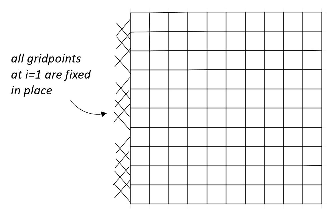
This tells FLAC the type of boundary condition (displacement-controlled) is applied at i=1 and that velocity is 0. at those gridpoints.
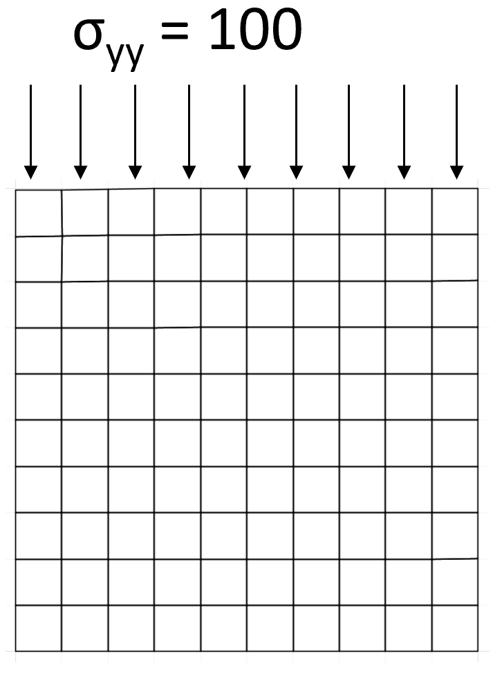
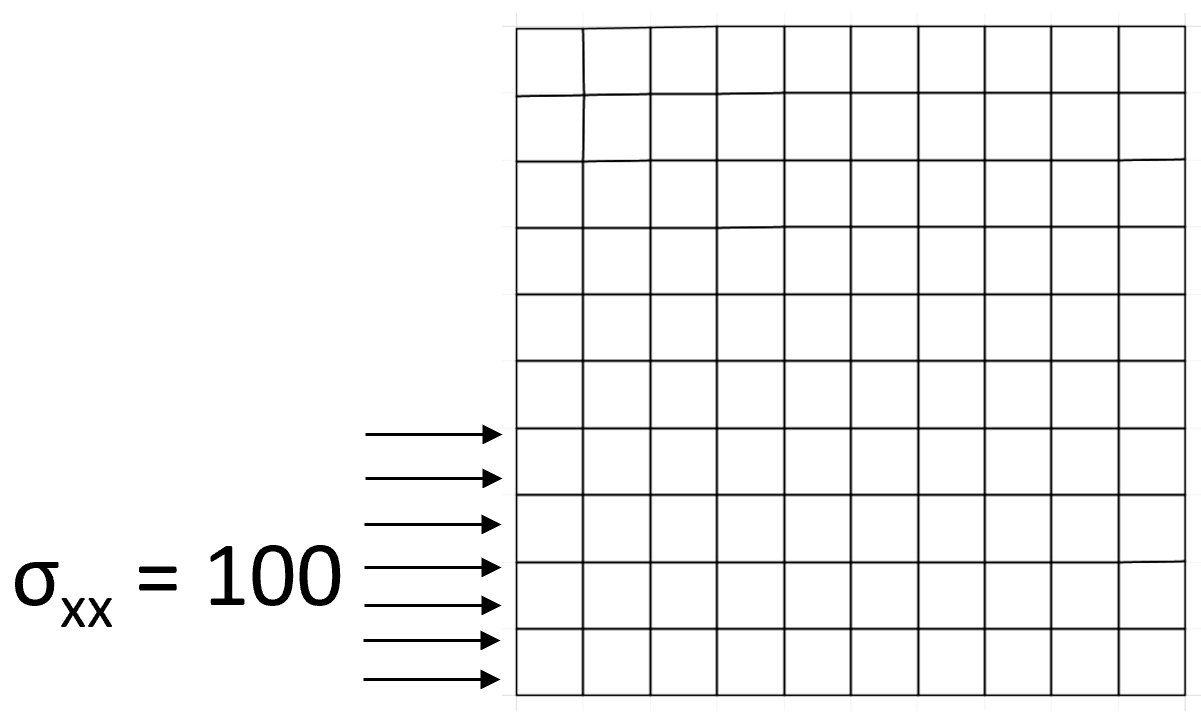
Stress-controlled boundaries can be applied along any boundary. The stress tensor components can be applied at a boundary (sxx for horizontal total stress, syy for vertical total stress, szz for out of plane stress, and sxy for shear stress).
The stress-controlled boundary is applied with the apply command in FLAC across gridpoints.
For example:
apply syy -100. j=11
apply sxx -50. i=1 i=1,5
Gradients at stress boundaries
Many geotechnical problems involve stress boundaries since vertical and horizontal stresses increase with depth. For a lot of this class we will not simulate problems with stress gradients, but the final assignment will require stress gradients.
To apply a stress gradient along a boundary, the var command is required.
apply sxx -200. var 0,200. from j=1,11 i=1
apply sxx -200. var 0,200. from j=1,11 i=11
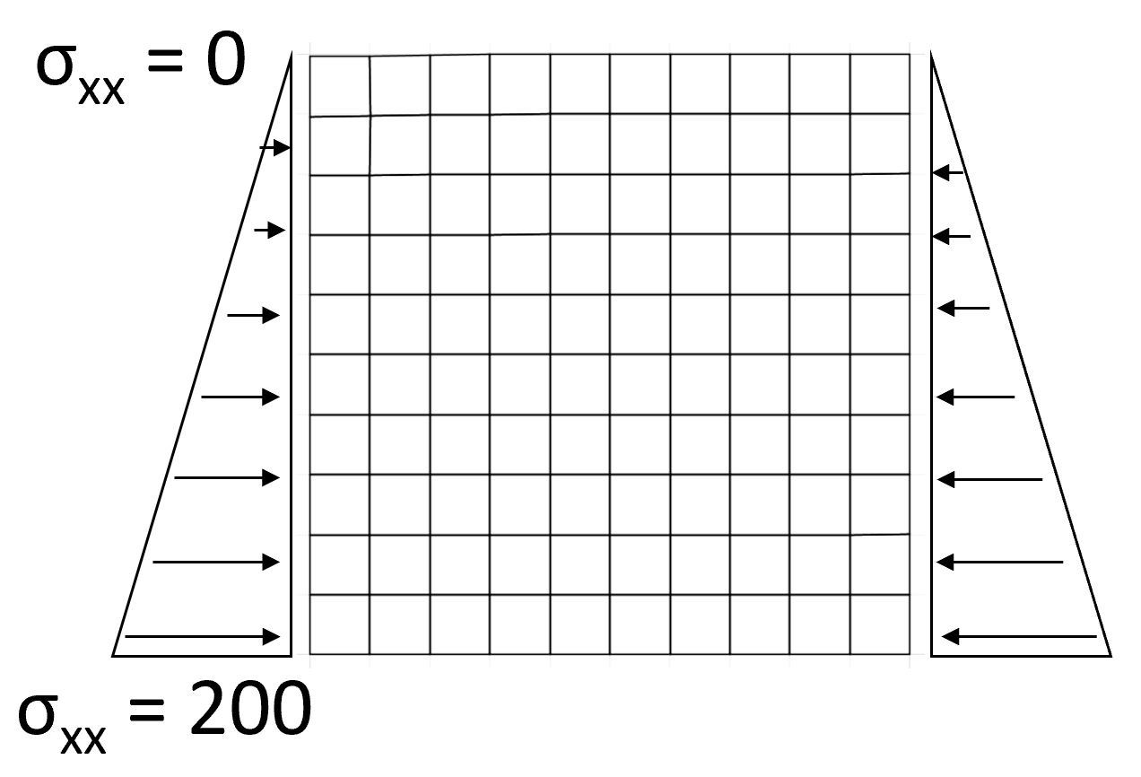
This command starts by applying sxx=200 at i=1 j=1 and i=11, j=1, then linearly increases sxx by 200 by the time the boundary reaches j=1.
There are a few things to keep in mind for assigning boundary conditions in FLAC:
- You cannot have a displacement boundary condition and stress boundary condition in the same direction for the same points. If this is assigned, the last command will supersede previous commands. For example, for the following commands, the boundary condition in the x-direction will be a displacement boundary condition.
app sxx $sxx i=1
ini xvel -1. i=1
- You can combine a displacement and stress-controlled boundary condition if they are in different directions. For example, the following boundary conditions for the j=1 boundary is permissible.
app syy $syy j=1
ini xvel 0.5 j=1
1D compression
These are example boundary conditions for 1D compression where the vertical stress is increased throughout the simulation.
A fish-function should be used to increase/decrease $syy throughout the simulation.
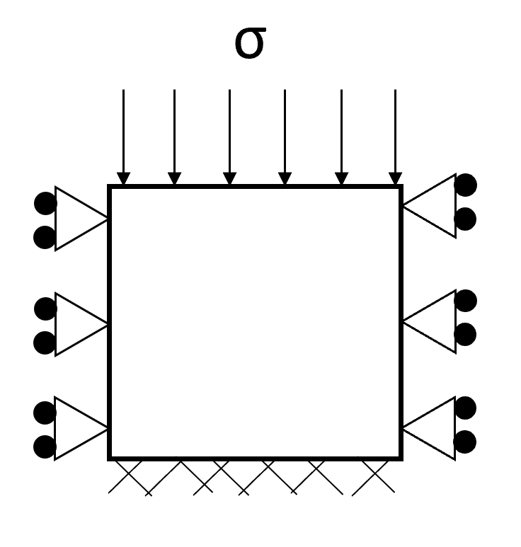
config axisymmetry

fix x y j=1
ini yvel 0. j=1
ini xvel 0. j=1

fix x i=1   ;;;not necessary bc/ axisymmetry

fix x i=gpi

apply syy $syy j=gpj
Isotropic compression
This example assumes axisymetric geometry for isotropic compression. The simulation takes an element from the isotropic compression test that is bounded by the radial symmetric and vertical symmetric boundaries.
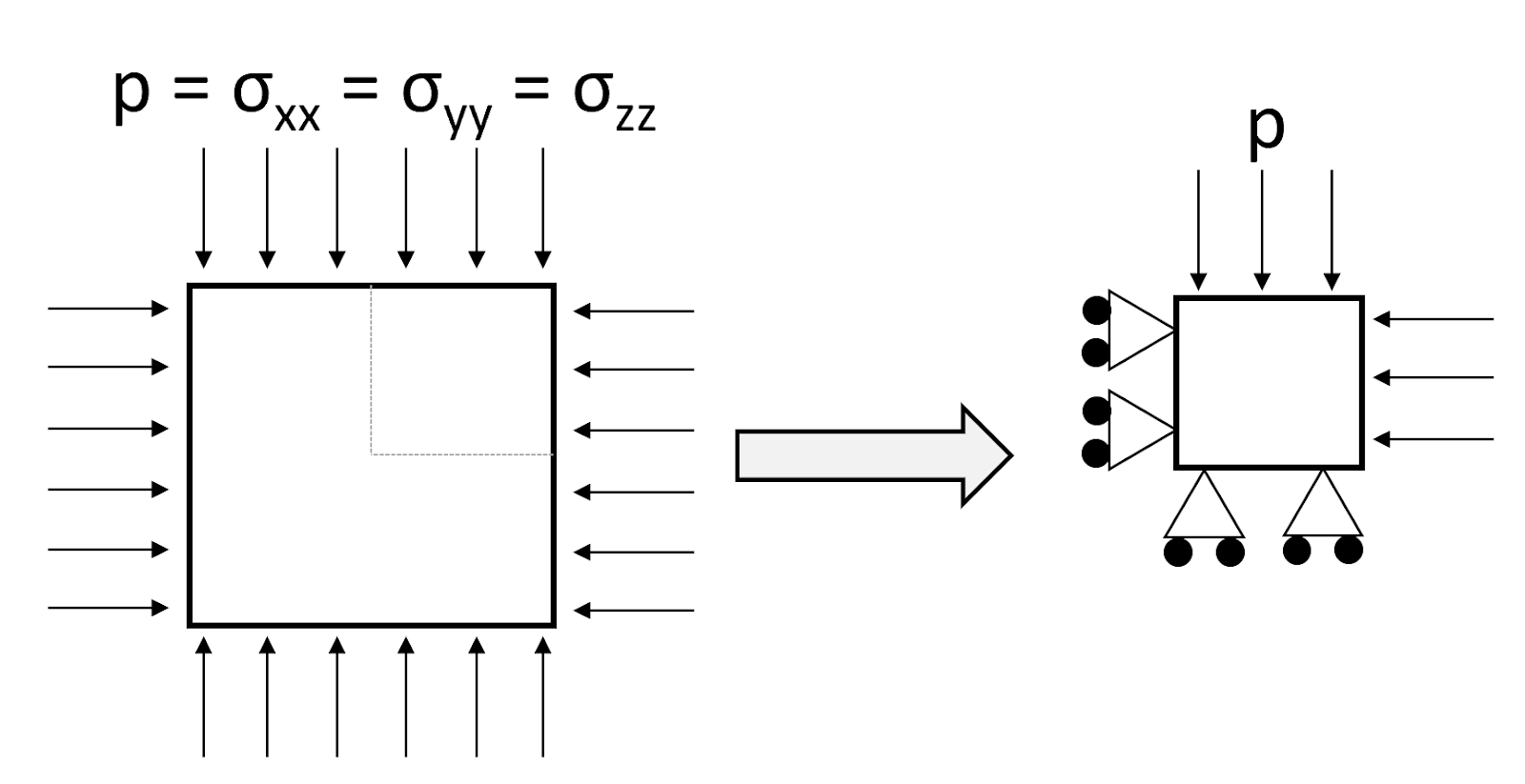
config axisymmetry

fix y j=1
fix x i=1   ;;;not necessary bc/ axisymmetry

apply sxx $p i=gpi
apply syy $p j=gpj
These commands assume that $p has been previously defined in a fish function.
Triaxial compression
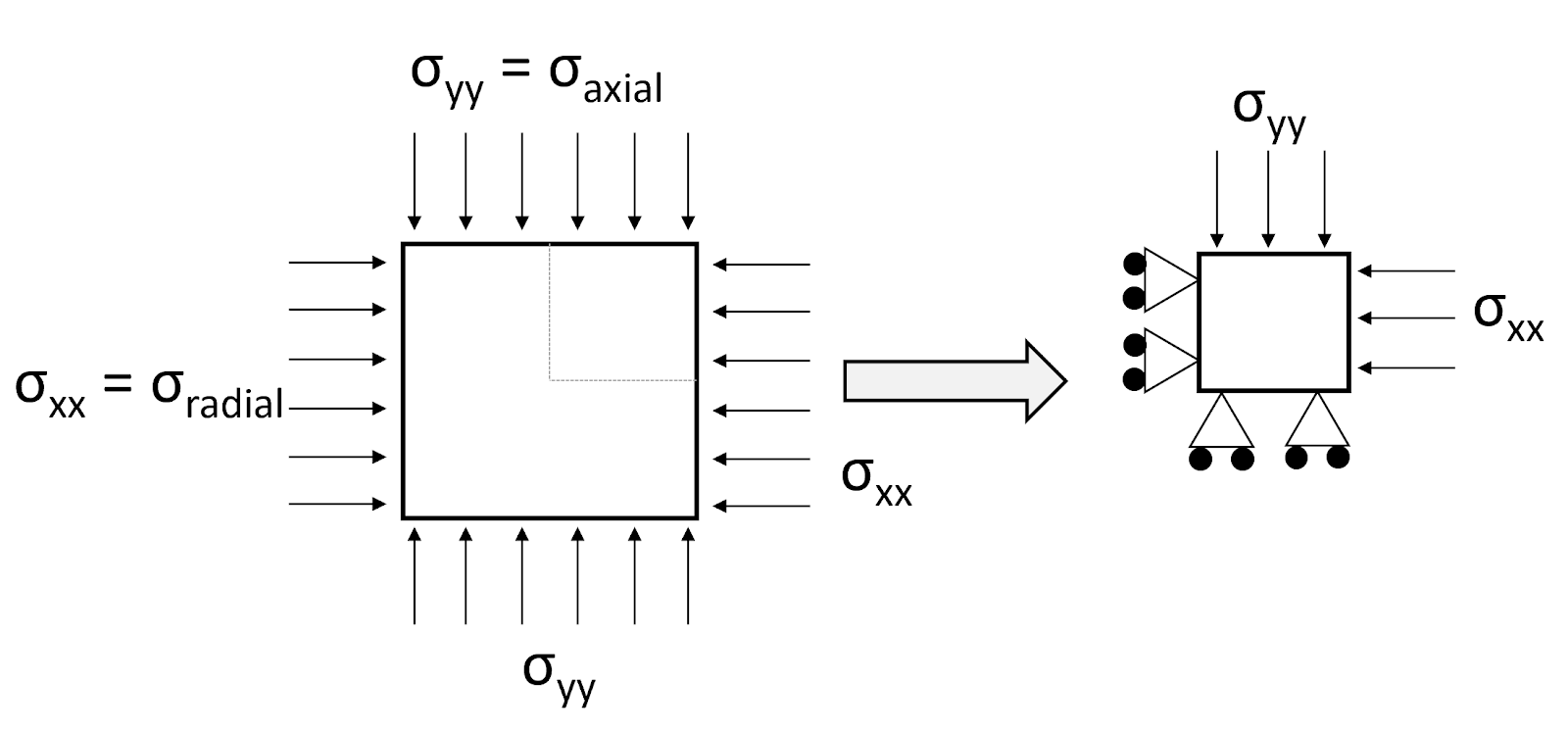
This example assumes axisymetric geometry. The simulation takes an element that is bounded from the radial symmetric boundary (the central axis) and the vertical symmetric boundary. Therefore, assuming this symmetry, the simulated element represents conditions throughout the test.
config axisymmetry

fix y j=1
fix x i=1   ;;;not necessary bc/ axisymmetry

apply sxx $sxx i=gpi
apply syy $syy j=gpj
These commands assume that $sxx and $syy were previously defined in a fish function.
Direct simple shear
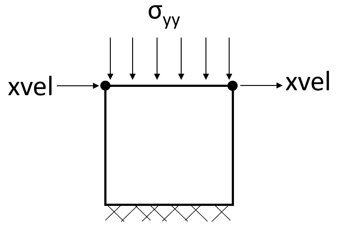
config

fix x y j=1
apply syy $syy j=gpj

fix x i=1 j=gpj
fix x i=gpi j=gpj

attach aside from 1,gpj to 1,1 bside from gpi,gpj to gpi,1
This introduces the attach command. The command in this case ensures that the two vertical boundaries move in-sync and keeps the constraint of no radial strain.